Blog Week 10
1. Open MATLAB. Open the editor and copy paste the following code. Name your code as FirstCode.m
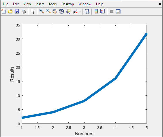 |
| Graph created by the code given in the blogsheet |
~~~~ Clears all predefined variables
3. What does close all do?
~~~~Closes all open windows such as graphs.
4. In the command line, type x and press enter. This is a matrix. How many rows and columns are there in the matrix?
~~~~ 1 row and zero columns
5. Why is there a semicolon at the end of the line of x and y?
~~~~ the semicolon prevents the data from being displayed after "ENTER" is hit.
6. Remove the dot on the y = 2.^x; line and execute the code again. What does the error message mean?
~~~~The dot is needed so that the operation can be applied to each of the values in the matrix
7. How does the LineWidth affect the plot? Explain.
~~~~ It affects the width of line. Smaller integers result in a more narrow line segment.
8. Type help plot on the command line and study the options for plot command. Provide how you would change the line for plot command to obtain the following figure (Hint: Like ‘LineWidth’, there is another property called ‘MarkerSize’)
~~~~plot(x,y,'LineWidth',6,'LineSpec',-or)
9. What happens if you change the line for x to x = [1; 2; 3; 4; 5]; ? Explain.
~~~~ It turns into a single column matrix starting at 1 and ending at 5
10. Provide the code for the following figure. You need to figure out the function for y. Notice there are grids on the plot.
x = [1 2 3 4 5];
y = x.^2;
plot(x, y,':sk', 'LineWidth', 6,'Markersize',20)
xlabel('Numbers', 'FontSize', 12)
ylabel('Results', 'FontSize', 12)
grid on
GridLineStyle ':'
11. Degree vs. radian in MATLAB:
a. Calculate sinus of 30 degrees using a calculator or internet.
Sin(30)= 1/2
b. Type sin(30) in the command line of the MATLAB. Why is this number different? (Hint: MATLAB treats angles as radians).
By default MatLab uses radians
c. How can you modify sin(30) so we get the correct number?
~~Sind(30)
12. Plot y = 10 sin (100 t) using Matlab with two different resolutions on the same plot: 10 points per period and 1000 points per period. The plot needs to show only two periods. Commands you might need to use are linspace, plot, hold on, legend, xlabel, and ylabel. Provide your code and resulting figure. The output figure should look like the following:
t=linspace(0,.125664,10);
y=10*sin(100*t);
plot(t,y,'-or')
hold on
clear t
t=linspace(0,.125664,1000);
y=10*sin(100*t);
plot(t,y,'k')
xlabel('Time (s)')
ylabel('y function')
legend('Coarse','Fine')
13. Explain what is changed in the following plot comparing to the previous one.
~~ The FINE graph has a limit set so that its max value is capped at 5
14. The command find was used to create this code. Study the use of find (help find) and try to replicate the plot above. Provide your code.
t=linspace(0,.125664,10);
y=10*sin(100*t);
plot(t,y,'-or')
hold on
clear t
t=linspace(0,.125664,1000);
y=10*sin(100*t);
k=find(y>5);
y(k)=5;
plot(t,y,'k')
xlabel('Time (s)')
ylabel('y function')
PART B: Filters and MATLAB
1. Build a low pass filter using a resistor and capacitor in which the cut off frequency is 1 kHz. Observe the output signal using the oscilloscope. Collect several data points particularly around the cut off frequency. Provide your data in a table.~~We need a 7.5k resistor to achieve a cutoff frequency of approximately 1kHz
| Table created from the frequency and the associated output in a low pass circuit |
2. Plot your data using MATLAB. Make sure to use proper labels for the plot and make your plot line and fonts readable. Provide your code and the plot.
 |
| Graph created from the table above. The code used is provided below |
****CODE*****
x=[.1 .2 .3 .4 .5 .6 .7 .8 .9 1 2 3];
y=[3.655 3.603 3.525 3.424 3.3 3.177 3.04 2.904 2.767 2.6 1.62 1.07];
plot(x,y)
xlabel('Freqency (KHz)');
ylabel('Vout (V)');
grid on
3. Calculate the cut off frequency using MATLAB. find command will be used. Provide your code.
R=7500; C=22*10^-9;
Cutoff=1/(2*pi*C*R)
----------------------> 964.5754 Hz
4. Put a horizontal dashed line on the previous plot that passes through the cutoff frequency.
 |
| Graph with dashed line across the cutoff point. This graph is identical to the graph above |
5. Repeat 1-3 by modifying the circuit to a high pass filter.
a)Table for high pass filter
| Table created by frequency and the associated output of a high pass filter circuit |
b)Graph for a high pass filter
 |
| Graph created from the table above. The code used is provided below |
***CODE***
%%
x=[.1 .2 .3 .4 .5 .6 .7 .8 .9 1 1.5 2 2.5 3];
y=[.35 .687 1.007 1.303 1.572 1.811 2.02 2.203 2.361 2.495 2.912 3.063 3.082 3.034];
plot(x,y)
xlabel('Freqency (KHz)');
ylabel('Vout (V)');
grid on
c)Calculate Cutoff of high pass filter
R=7500; C=22*10^-9;
Cutoff=1/(2*pi*C*R)
----------------------> 964.5754 Hz
~~This cutoff is the same for both low pass and high pass filter.
The blog is good, the only thing is that the code being copied and pasted without syntax highlighting makes it a bit look off and hard to read.
ReplyDeleteYour data looks good, but I would have liked to see more graphs, as the visuals of what the program is doing in the 2-D space help to envision what the actual code is trying to accomplish.
ReplyDeleteFor your answers from 10 to 14 on part A, you have good info, but when reading it there are no examples of what that code created, plots made. Some of those could go a long way.
ReplyDeleteFor your answers from 10 to 14 on part A, you have good info, but when reading it there are no examples of what that code created, plots made. Some of those could go a long way.
ReplyDeleteno response to comments.
ReplyDelete